Reintroducing the tidyverse

Readings

This page.
Chapter 1 of Introduction to Statistical Learning, available here.
Optional: The “Tidy Your Data” tutorial on Rstudio Cloud Primers

Your labs

Start labs early!
- They are not trivial.
- They are not short.
- They are not easy.
- They are not optional.
You install.packages("packageName") once on your computer.
- And never ever ever in your code.
You load an already-installed package using library(packageName) in a code chunk
- Never in your console
- When RMarkdown knits, it starts a whole new, empty session that has no knowledge of what you typed into the console
Slack
- Use it.
- Always post in the class-visible channels. Others can learn from your issues.
  - We have a channel just for labs and R. Please use that one.

Group project

If you read ahead, you’d have seen a bit about our group project. I’d like to wait until after the add/drop deadline to do this as people come and go, ruining my group assignments. Know that we will have groups of 3, and you will be given the opportunity to form your own groups with default groups for those who do not form one. All groups must be exactly 3 people.

Guiding Question

For future lectures, the guiding questions will be more pointed and at a higher level to help steer your thinking. Here, we want to ensure you remember some basics and accordingly the questions are straightforward.

Why do we want tidy data?
What are the challenges associated with shaping things into a tidy format?

The tidyverse

You should already be familiar with the Tidyverse, including filter, select and %>%. If not, click here to expand material.

In last week’s content and lab, we demonstrated how to manipulate vectors by reordering and subsetting them through indexing. However, once we start more advanced analyses, the preferred unit for data storage is not the vector but the data frame. In this lecture, we learn to work directly with data frames, which greatly facilitate the organization of information. We will be using data frames for the majority of this class and you will use them for the majority of your data science life (however long that might be). We will focus on a specific data format referred to as tidy and on specific collection of packages that are particularly helpful for working with tidy data referred to as the tidyverse.

We can load all the tidyverse packages at once by installing and loading the tidyverse package:¹

library(tidyverse)

We will learn how to implement the tidyverse approach throughout the book, but before delving into the details, in this chapter we introduce some of the most widely used tidyverse functionality, starting with the dplyr package for manipulating data frames and the purrr package for working with functions. Note that the tidyverse also includes a graphing package, ggplot2, the readr package, and many others. In this lesson, we first introduce the concept of tidy data and then demonstrate how we use the tidyverse to work with data frames in this format.

Tidy data

We say that a data table is in tidy format if each row represents one observation and columns represent the different variables available for each of these observations. The murders dataset is an example of a tidy data frame.

library(dslabs)
data(murders)
head(murders)

       state abb region population total
1    Alabama  AL  South    4779736   135
2     Alaska  AK   West     710231    19
3    Arizona  AZ   West    6392017   232
4   Arkansas  AR  South    2915918    93
5 California  CA   West   37253956  1257
6   Colorado  CO   West    5029196    65

Each row represent a state with each of the five columns providing a different variable related to these states: name, abbreviation, region, population, and total murders.

To see how the same information can be provided in different formats, consider the following example:

      country year fertility
1     Germany 1960      2.41
2 South Korea 1960      6.16
3     Germany 1961      2.44
4 South Korea 1961      5.99
5     Germany 1962      2.47
6 South Korea 1962      5.79

This tidy dataset provides fertility rates for two countries across the years. This is a tidy dataset because each row presents one observation with the three variables being country, year, and fertility rate. However, this dataset originally came in another format and was reshaped for the dslabs package. Originally, the data was in the following format:

      country 1960 1961 1962
1     Germany 2.41 2.44 2.47
2 South Korea 6.16 5.99 5.79

The same information is provided, but there are two important differences in the format: 1) each row includes several observations and 2) one of the variables’ values, year, is stored in the header. For the tidyverse packages to be optimally used, data need to be reshaped into tidy format, which you will learn to do throughout this course. For starters, though, we will use example datasets that are already in tidy format.

Although not immediately obvious, as you go through the book you will start to appreciate the advantages of working in a framework in which functions use tidy formats for both inputs and outputs. You will see how this permits the data analyst to focus on more important aspects of the analysis rather than the format of the data.

TRY IT

Examine the built-in dataset co2. Which of the following is true:

co2 is tidy data: it has one year for each row.
co2 is not tidy: we need at least one column with a character vector.
co2 is not tidy: it is a matrix instead of a data frame.
co2 is not tidy: to be tidy we would have to wrangle it to have three columns (year, month and value), then each co2 observation would have a row.

Examine the built-in dataset ChickWeight. Which of the following is true:

ChickWeight is not tidy: each chick has more than one row.
ChickWeight is tidy: each observation (a weight) is represented by one row. The chick from which this measurement came is one of the variables.
ChickWeight is not tidy: we are missing the year column.
ChickWeight is tidy: it is stored in a data frame.

Examine the built-in dataset BOD. Which of the following is true:

BOD is not tidy: it only has six rows.
BOD is not tidy: the first column is just an index.
BOD is tidy: each row is an observation with two values (time and demand)
BOD is tidy: all small datasets are tidy by definition.

Which of the following built-in datasets is tidy (you can pick more than one):

BJsales
EuStockMarkets
DNase
Formaldehyde
Orange
UCBAdmissions

Manipulating data frames

The dplyr package from the tidyverse introduces functions that perform some of the most common operations when working with data frames and uses names for these functions that are relatively easy to remember. For instance, to change the data table by adding a new column, we use mutate. To filter the data table to a subset of rows, we use filter. Finally, to subset the data by selecting specific columns, we use select.

Adding a column with `mutate`

We want all the necessary information for our analysis to be included in the data table. So the first task is to add the murder rates to our murders data frame. The function mutate takes the data frame as a first argument and the name and values of the variable as a second argument using the convention name = values. So, to add murder rates, we use:

library(dslabs)
data("murders")
murders <- mutate(murders, rate = total / population * 100000)

Notice that here we used total and population inside the function, which are objects that are not defined in our workspace. But why don’t we get an error?

This is one of dplyr’s main features. Functions in this package, such as mutate, know to look for variables in the data frame provided in the first argument. In the call to mutate above, total will have the values in murders$total. This approach makes the code much more readable.

We can see that the new column is added:

head(murders)

       state abb region population total     rate
1    Alabama  AL  South    4779736   135 2.824424
2     Alaska  AK   West     710231    19 2.675186
3    Arizona  AZ   West    6392017   232 3.629527
4   Arkansas  AR  South    2915918    93 3.189390
5 California  CA   West   37253956  1257 3.374138
6   Colorado  CO   West    5029196    65 1.292453

Note: Although we have overwritten the original murders object, this does not change the object that loaded with data(murders). If we load the murders data again, the original will overwrite our mutated version.

Subsetting with `filter`

Now suppose that we want to filter the data table to only show the entries for which the murder rate is lower than 0.71. To do this we use the filter function, which takes the data table as the first argument and then the conditional statement as the second. Like mutate, we can use the unquoted variable names from murders inside the function and it will know we mean the columns and not objects in the workspace.

filter(murders, rate <= 0.71)

          state abb        region population total      rate
1        Hawaii  HI          West    1360301     7 0.5145920
2          Iowa  IA North Central    3046355    21 0.6893484
3 New Hampshire  NH     Northeast    1316470     5 0.3798036
4  North Dakota  ND North Central     672591     4 0.5947151
5       Vermont  VT     Northeast     625741     2 0.3196211

Selecting columns with `select`

Although our data table only has six columns, some data tables include hundreds. If we want to view just a few, we can use the dplyr select function. In the code below we select three columns, assign this to a new object and then filter the new object:

new_table <- select(murders, state, region, rate)
filter(new_table, rate <= 0.71)

          state        region      rate
1        Hawaii          West 0.5145920
2          Iowa North Central 0.6893484
3 New Hampshire     Northeast 0.3798036
4  North Dakota North Central 0.5947151
5       Vermont     Northeast 0.3196211

In the call to select, the first argument murders is an object, but state, region, and rate are variable names.

TRY IT

Load the dplyr package and the murders dataset.

library(dplyr)
library(dslabs)
data(murders)

You can add columns using the dplyr function mutate. This function is aware of the column names and inside the function you can call them unquoted:

murders <- mutate(murders, population_in_millions = population / 10^6)

We can write population rather than murders$population because mutate is part of dplyr. The function mutate knows we are grabbing columns from murders.

Use the function mutate to add a murders column named rate with the per 100,000 murder rate as in the example code above. Make sure you redefine murders as done in the example code above ( murders <- [your code]) so we can keep using this variable.

If rank(x) gives you the ranks of x from lowest to highest, rank(-x) gives you the ranks from highest to lowest. Use the function mutate to add a column rank containing the rank, from highest to lowest murder rate. Make sure you redefine murders so we can keep using this variable.
With dplyr, we can use select to show only certain columns. For example, with this code we would only show the states and population sizes:

select(murders, state, population) %>% head()

Use select to show the state names and abbreviations in murders. Do not redefine murders, just show the results.

The dplyr function filter is used to choose specific rows of the data frame to keep. Unlike select which is for columns, filter is for rows. For example, you can show just the New York row like this:

filter(murders, state == "New York")

You can use other logical vectors to filter rows.

Use filter to show the top 5 states with the highest murder rates. After we add murder rate and rank, do not change the murders dataset, just show the result. Remember that you can filter based on the rank column.

We can remove rows using the != operator. For example, to remove Florida, we would do this:

no_florida <- filter(murders, state != "Florida")

Create a new data frame called no_south that removes states from the South region. How many states are in this category? You can use the function nrow for this.

We can also use %in% to filter with dplyr. You can therefore see the data from New York and Texas like this:

filter(murders, state %in% c("New York", "Texas"))

Create a new data frame called murders_nw with only the states from the Northeast and the West. How many states are in this category?

Suppose you want to live in the Northeast or West and want the murder rate to be less than 1. We want to see the data for the states satisfying these options. Note that you can use logical operators with filter. Here is an example in which we filter to keep only small states in the Northeast region.

filter(murders, population < 5000000 & region == "Northeast")

Make sure murders has been defined with rate and rank and still has all states. Create a table called my_states that contains rows for states satisfying both the conditions: it is in the Northeast or West and the murder rate is less than 1. Use select to show only the state name, the rate, and the rank.

The pipe: `%>%`

With dplyr we can perform a series of operations, for example select and then filter, by sending the results of one function to another using what is called the pipe operator: %>%. Some details are included below.

We wrote code above to show three variables (state, region, rate) for states that have murder rates below 0.71. To do this, we defined the intermediate object new_table. In dplyr we can write code that looks more like a description of what we want to do without intermediate objects:

\[ \mbox{original data } \rightarrow \mbox{ select } \rightarrow \mbox{ filter } \]

For such an operation, we can use the pipe %>%. The code looks like this:

murders %>% select(state, region, rate) %>% filter(rate <= 0.71)

          state        region      rate
1        Hawaii          West 0.5145920
2          Iowa North Central 0.6893484
3 New Hampshire     Northeast 0.3798036
4  North Dakota North Central 0.5947151
5       Vermont     Northeast 0.3196211

This line of code is equivalent to the two lines of code above. What is going on here?

In general, the pipe sends the result of the left side of the pipe to be the first argument of the function on the right side of the pipe. Here is a very simple example:

16 %>% sqrt()

[1] 4

We can continue to pipe values along:

16 %>% sqrt() %>% log2()

[1] 2

The above statement is equivalent to log2(sqrt(16)).

Remember that the pipe sends values to the first argument, so we can define other arguments as if the first argument is already defined:

16 %>% sqrt() %>% log(base = 2)

[1] 2

Therefore, when using the pipe with data frames and dplyr, we no longer need to specify the required first argument since the dplyr functions we have described all take the data as the first argument. In the code we wrote:

murders %>% select(state, region, rate) %>% filter(rate <= 0.71)

murders is the first argument of the select function, and the new data frame (formerly new_table) is the first argument of the filter function.

Note that the pipe works well with functions where the first argument is the input data. Functions in tidyverse packages like dplyr have this format and can be used easily with the pipe. It’s worth noting that as of R 4.1, there is a base-R version of the pipe |>, though this has its disadvantages. We’ll stick with %>% for now.

TRY IT

The pipe %>% can be used to perform operations sequentially without having to define intermediate objects. Start by redefining murder to include rate and rank.

murders <- mutate(murders, rate =  total / population * 100000,
                  rank = rank(-rate))

In the solution to the previous exercise, we did the following:

my_states <- filter(murders, region %in% c("Northeast", "West") &
                      rate < 1)

select(my_states, state, rate, rank)

The pipe %>% permits us to perform both operations sequentially without having to define an intermediate variable my_states. We therefore could have mutated and selected in the same line like this:

mutate(murders, rate =  total / population * 100000,
       rank = rank(-rate)) %>%
  select(state, rate, rank)

Notice that select no longer has a data frame as the first argument. The first argument is assumed to be the result of the operation conducted right before the %>%.

Repeat the previous exercise, but now instead of creating a new object, show the result and only include the state, rate, and rank columns. Use a pipe %>% to do this in just one line.

Reset murders to the original table by using data(murders). Use a pipe to create a new data frame called my_states that considers only states in the Northeast or West which have a murder rate lower than 1, and contains only the state, rate and rank columns. The pipe should also have four components separated by three %>%. The code should look something like this:

my_states <- murders %>%
  mutate SOMETHING %>%
  filter SOMETHING %>%
  select SOMETHING

Summarizing data

An important part of exploratory data analysis is summarizing data. The average and standard deviation are two examples of widely used summary statistics. More informative summaries can often be achieved by first splitting data into groups. In this section, we cover two new dplyr verbs that make these computations easier: summarize and group_by. We learn to access resulting values using the pull function.

`summarize`

The summarize function in dplyr provides a way to compute summary statistics with intuitive and readable code. We start with a simple example based on heights. The heights dataset includes heights and sex reported by students in an in-class survey.

library(dplyr)
library(dslabs)
data(heights)
head(heights)

     sex height
1   Male     75
2   Male     70
3   Male     68
4   Male     74
5   Male     61
6 Female     65

The following code computes the average and standard deviation for females:

s <- heights %>%
  filter(sex == "Female") %>%
  summarize(average = mean(height), standard_deviation = sd(height))
s

   average standard_deviation
1 64.93942           3.760656

This takes our original data table as input, filters it to keep only females, and then produces a new summarized table with just the average and the standard deviation of heights. We get to choose the names of the columns of the resulting table. For example, above we decided to use average and standard_deviation, but we could have used other names just the same.

Because the resulting table stored in s is a data frame, we can access the components with the accessor $:

s$average

[1] 64.93942

s$standard_deviation

[1] 3.760656

As with most other dplyr functions, summarize is aware of the variable names and we can use them directly. So when inside the call to the summarize function we write mean(height), the function is accessing the column with the name “height” and then computing the average of the resulting numeric vector. We can compute any other summary that operates on vectors and returns a single value. For example, we can add the median, minimum, and maximum heights like this:

heights %>%
  filter(sex == "Female") %>%
  summarize(median = median(height), minimum = min(height),
            maximum = max(height))

    median minimum maximum
1 64.98031      51      79

We can obtain these three values with just one line using the quantile function: for example, quantile(x, c(0,0.5,1)) returns the min (0th percentile), median (50th percentile), and max (100th percentile) of the vector x. However, if we attempt to use a function like this that returns two or more values inside summarize:

heights %>%
  filter(sex == "Female") %>%
  summarize(range = quantile(height, c(0, 0.5, 1)))

we will receive an error: Error: expecting result of length one, got : 2. With the function summarize, we can only call functions that return a single value. In later sections, we will learn how to deal with functions that return more than one value.

For another example of how we can use the summarize function, let’s compute the average murder rate for the United States. Remember our data table includes total murders and population size for each state and we have already used dplyr to add a murder rate column:

murders <- murders %>% mutate(rate = total/population*100000)

Remember that the US murder rate is not the average of the state murder rates:

summarize(murders, mean(rate))

  mean(rate)
1   2.779125

This is because in the computation above the small states are given the same weight as the large ones. The US murder rate is the total number of murders in the US divided by the total US population. So the correct computation is:

us_murder_rate <- murders %>%
  summarize(rate = sum(total) / sum(population) * 100000)
us_murder_rate

      rate
1 3.034555

This computation counts larger states proportionally to their size which results in a larger value.

`pull`

The us_murder_rate object defined above represents just one number. Yet we are storing it in a data frame:

class(us_murder_rate)

[1] "data.frame"

since, as most dplyr functions, summarize always returns a data frame.

This might be problematic if we want to use this result with functions that require a numeric value. Here we show a useful trick for accessing values stored in data when using pipes: when a data object is piped that object and its columns can be accessed using the pull function. To understand what we mean take a look at this line of code:

us_murder_rate %>% pull(rate)

[1] 3.034555

This returns the value in the rate column of us_murder_rate making it equivalent to us_murder_rate$rate.

To get a number from the original data table with one line of code we can type:

us_murder_rate <- murders %>%
  summarize(rate = sum(total) / sum(population) * 100000) %>%
  pull(rate)

us_murder_rate

[1] 3.034555

which is now a numeric:

class(us_murder_rate)

[1] "numeric"

Group then summarize with `group_by`

A common operation in data exploration is to first split data into groups and then compute summaries for each group. For example, we may want to compute the average and standard deviation for men’s and women’s heights separately. The group_by function helps us do this.

If we type this:

heights %>% group_by(sex)

# A tibble: 1,050 × 2
# Groups:   sex [2]
   sex    height
   <fct>   <dbl>
 1 Male       75
 2 Male       70
 3 Male       68
 4 Male       74
 5 Male       61
 6 Female     65
 7 Female     66
 8 Female     62
 9 Female     66
10 Male       67
# ℹ 1,040 more rows

The result does not look very different from heights, except we see Groups: sex [2] when we print the object. Although not immediately obvious from its appearance, this is now a special data frame called a grouped data frame, and dplyr functions, in particular summarize, will behave differently when acting on this object. Conceptually, you can think of this table as many tables, with the same columns but not necessarily the same number of rows, stacked together in one object. When we summarize the data after grouping, this is what happens:

heights %>%
  group_by(sex) %>%
  summarize(average = mean(height), standard_deviation = sd(height))

# A tibble: 2 × 3
  sex    average standard_deviation
  <fct>    <dbl>              <dbl>
1 Female    64.9               3.76
2 Male      69.3               3.61

The summarize function applies the summarization to each group separately.

For another example, let’s compute the median murder rate in the four regions of the country:

murders %>%
  group_by(region) %>%
  summarize(median_rate = median(rate))

# A tibble: 4 × 2
  region        median_rate
  <fct>               <dbl>
1 Northeast            1.80
2 South                3.40
3 North Central        1.97
4 West                 1.29

Sorting data frames

When examining a dataset, it is often convenient to sort the table by the different columns. We know about the order and sort function, but for ordering entire tables, the dplyr function arrange is useful. For example, here we order the states by population size:

murders %>%
  arrange(population) %>%
  head()

                 state abb        region population total       rate
1              Wyoming  WY          West     563626     5  0.8871131
2 District of Columbia  DC         South     601723    99 16.4527532
3              Vermont  VT     Northeast     625741     2  0.3196211
4         North Dakota  ND North Central     672591     4  0.5947151
5               Alaska  AK          West     710231    19  2.6751860
6         South Dakota  SD North Central     814180     8  0.9825837

With arrange we get to decide which column to sort by. To see the states by murder rate, from lowest to highest, we arrange by rate instead:

murders %>%
  arrange(rate) %>%
  head()

          state abb        region population total      rate
1       Vermont  VT     Northeast     625741     2 0.3196211
2 New Hampshire  NH     Northeast    1316470     5 0.3798036
3        Hawaii  HI          West    1360301     7 0.5145920
4  North Dakota  ND North Central     672591     4 0.5947151
5          Iowa  IA North Central    3046355    21 0.6893484
6         Idaho  ID          West    1567582    12 0.7655102

Note that the default behavior is to order in ascending order. In dplyr, the function desc transforms a vector so that it is in descending order. To sort the table in descending order, we can type:

murders %>%
  arrange(desc(rate))

Nested sorting

If we are ordering by a column with ties, we can use a second column to break the tie. Similarly, a third column can be used to break ties between first and second and so on. Here we order by region, then within region we order by murder rate:

murders %>%
  arrange(region, rate) %>%
  head()

          state abb    region population total      rate
1       Vermont  VT Northeast     625741     2 0.3196211
2 New Hampshire  NH Northeast    1316470     5 0.3798036
3         Maine  ME Northeast    1328361    11 0.8280881
4  Rhode Island  RI Northeast    1052567    16 1.5200933
5 Massachusetts  MA Northeast    6547629   118 1.8021791
6      New York  NY Northeast   19378102   517 2.6679599

TRY IT

For these exercises, we will be using the data from the survey collected by the United States National Center for Health Statistics (NCHS). This center has conducted a series of health and nutrition surveys since the 1960’s. Starting in 1999, about 5,000 individuals of all ages have been interviewed every year and they complete the health examination component of the survey. Part of the data is made available via the NHANES package. Once you install the NHANES package, you can load the data like this:

library(NHANES)
data(NHANES)

The NHANES data has many missing values. The mean and sd functions in R will return NA if any of the entries of the input vector is an NA. Here is an example:

library(dslabs)
data(na_example)
mean(na_example)

[1] NA

sd(na_example)

[1] NA

To ignore the NAs we can use the na.rm argument:

mean(na_example, na.rm = TRUE)

[1] 2.301754

sd(na_example, na.rm = TRUE)

[1] 1.22338

Let’s now explore the NHANES data.

We will provide some basic facts about blood pressure. First let’s select a group to set the standard. We will use 20-to-29-year-old females. AgeDecade is a categorical variable with these ages. Note that the category is coded like ” 20-29”, with a space in front! What is the average and standard deviation of systolic blood pressure as saved in the BPSysAve variable? Save it to a variable called ref.

Hint: Use filter and summarize and use the na.rm = TRUE argument when computing the average and standard deviation. You can also filter the NA values using filter.

Using a pipe, assign the average to a numeric variable ref_avg. Hint: Use the code similar to above and then pull.
Now report the min and max values for the same group.
Compute the average and standard deviation for females, but for each age group separately rather than a selected decade as in question 1. Note that the age groups are defined by AgeDecade. Hint: rather than filtering by age and gender, filter by Gender and then use group_by.
Repeat exercise 4 for males.
We can actually combine both summaries for exercises 4 and 5 into one line of code. This is because group_by permits us to group by more than one variable. Obtain one big summary table using group_by(AgeDecade, Gender).
For males between the ages of 40-49, compare systolic blood pressure across race as reported in the Race1 variable. Order the resulting table from lowest to highest average systolic blood pressure.

Tibbles

Tidy data must be stored in data frames. We have been using the murders data frame throughout the unit. In an earlier section we introduced the group_by function, which permits stratifying data before computing summary statistics. But where is the group information stored in the data frame?

murders %>% group_by(region)

# A tibble: 51 × 6
# Groups:   region [4]
   state                abb   region    population total  rate
   <chr>                <chr> <fct>          <dbl> <dbl> <dbl>
 1 Alabama              AL    South        4779736   135  2.82
 2 Alaska               AK    West          710231    19  2.68
 3 Arizona              AZ    West         6392017   232  3.63
 4 Arkansas             AR    South        2915918    93  3.19
 5 California           CA    West        37253956  1257  3.37
 6 Colorado             CO    West         5029196    65  1.29
 7 Connecticut          CT    Northeast    3574097    97  2.71
 8 Delaware             DE    South         897934    38  4.23
 9 District of Columbia DC    South         601723    99 16.5 
10 Florida              FL    South       19687653   669  3.40
# ℹ 41 more rows

Notice that there are no columns with this information. But, if you look closely at the output above, you see the line A tibble followed by dimensions. We can learn the class of the returned object using:

murders %>% group_by(region) %>% class()

[1] "grouped_df" "tbl_df"     "tbl"        "data.frame"

The tbl, pronounced tibble, is a special kind of data frame. The functions group_by and summarize always return this type of data frame. The group_by function returns a special kind of tbl, the grouped_df. We will say more about these later. For consistency, the dplyr manipulation verbs (select, filter, mutate, and arrange) preserve the class of the input: if they receive a regular data frame they return a regular data frame, while if they receive a tibble they return a tibble. But tibbles are the preferred format in the tidyverse and as a result tidyverse functions that produce a data frame from scratch return a tibble.

Tibbles are very similar to data frames. In fact, you can think of them as a modern version of data frames. Nonetheless there are three important differences which we describe next.

Tibbles display better

The print method for tibbles is more readable than that of a data frame. To see this, compare the outputs of typing murders and the output of murders if we convert it to a tibble. We can do this using as_tibble(murders). If using RStudio, output for a tibble adjusts to your window size. To see this, change the width of your R console and notice how more/less columns are shown.

Tibbles can be grouped

The function group_by returns a special kind of tibble: a grouped tibble. This class stores information that lets you know which rows are in which groups. The tidyverse functions, in particular the summarize function, are aware of the group information.

Create a tibble using `tibble` instead of `data.frame`

It is sometimes useful for us to create our own data frames. To create a data frame in the tibble format, you can do this by using the tibble function.

grades <- tibble(names = c("John", "Juan", "Jean", "Yao"),
                     exam_1 = c(95, 80, 90, 85),
                     exam_2 = c(90, 85, 85, 90))

Note that base R (without packages loaded) has a function with a very similar name, data.frame, that can be used to create a regular data frame rather than a tibble. One other important difference is that by default data.frame coerces characters into factors without providing a warning or message:

grades <- data.frame(names = c("John", "Juan", "Jean", "Yao"),
                     exam_1 = c(95, 80, 90, 85),
                     exam_2 = c(90, 85, 85, 90))
class(grades$names)

[1] "character"

To avoid this, we use the rather cumbersome argument stringsAsFactors:

grades <- data.frame(names = c("John", "Juan", "Jean", "Yao"),
                     exam_1 = c(95, 80, 90, 85),
                     exam_2 = c(90, 85, 85, 90),
                     stringsAsFactors = FALSE)
class(grades$names)

[1] "character"

To convert a regular data frame to a tibble, you can use the as_tibble function.

as_tibble(grades) %>% class()

[1] "tbl_df"     "tbl"        "data.frame"

Applying more complex functions

The dot operator

One of the advantages of using the pipe %>% is that we do not have to keep naming new objects as we manipulate the data frame. As a quick reminder, if we want to compute the median murder rate for states in the southern states, instead of typing:

tab_1 <- filter(murders, region == "South")
tab_2 <- mutate(tab_1, rate = total / population * 10^5)
rates <- tab_2$rate
median(rates)

[1] 3.398069

We can avoid defining any new intermediate objects by instead typing:

filter(murders, region == "South") %>%
  mutate(rate = total / population * 10^5) %>%
  summarize(median = median(rate)) %>%
  pull(median)

[1] 3.398069

We can do this because each of these functions takes a data frame as the first argument. But what if we want to access a component of the data frame. For example, what if the pull function was not available and we wanted to access tab_2$rate? What data frame name would we use? The answer is the dot operator.

For example to access the rate vector without the pull function we could use

rates <-   filter(murders, region == "South") %>%
  mutate(rate = total / population * 10^5) %>%
  .$rate
median(rates)

[1] 3.398069

The purrr package

In previous sections (and labs) we learned about the sapply function, which permitted us to apply the same function to each element of a vector. We constructed a function and used sapply to compute the sum of the first n integers for several values of n like this:

compute_s_n <- function(n){
  x <- 1:n
  sum(x)
}
n <- 1:25
s_n <- sapply(n, compute_s_n)
s_n

 [1]   1   3   6  10  15  21  28  36  45  55  66  78  91 105 120 136 153 171 190
[20] 210 231 253 276 300 325

This type of operation, applying the same function or procedure to elements of an object, is quite common in data analysis. The purrr package includes functions similar to sapply but that better interact with other tidyverse functions. The main advantage is that we can better control the output type of functions. In contrast, sapply can return several different object types; for example, we might expect a numeric result from a line of code, but sapply might convert our result to character under some circumstances. purrr functions will never do this: they will return objects of a specified type or return an error if this is not possible.

The first purrr function we will learn is map, which works very similar to sapply but always, without exception, returns a list:

library(purrr) # or library(tidyverse)
n <- 1:25
s_n <- map(n, compute_s_n)
class(s_n)

[1] "list"

If we want a numeric vector, we can instead use map_dbl which always returns a vector of numeric values.

s_n <- map_dbl(n, compute_s_n)
class(s_n)

[1] "numeric"

This produces the same results as the sapply call shown above.

A particularly useful purrr function for interacting with the rest of the tidyverse is map_df, which always returns a tibble data frame. However, the function being called needs to return a vector, a tibble, or a list with names. For this reason, the following code would result in a Argument 1 must have names error:

s_n <- map_df(n, compute_s_n)

We need to change the function to make this work:

compute_s_n <- function(n){
  x <- 1:n
  tibble(sum = sum(x))
}
s_n <- map_df(n, compute_s_n)
head(s_n)

# A tibble: 6 × 1
    sum
  <int>
1     1
2     3
3     6
4    10
5    15
6    21

Because map_df returns a tibble, we can have more columns defined in our function and returned.

compute_s_n2 <- function(n){
  x <- 1:n
  tibble(sum = sum(x), sumSquared = sum(x^2))
}
s_n <- map_df(n, compute_s_n2)
head(s_n)

# A tibble: 6 × 2
    sum sumSquared
  <int>      <dbl>
1     1          1
2     3          5
3     6         14
4    10         30
5    15         55
6    21         91

The purrr package provides much more functionality not covered here. For more details you can consult this online resource.

Tidyverse conditionals

A typical data analysis will often involve one or more conditional operations. You should be familiar with the ifelse function, which we will use extensively in this course In this section we present two dplyr functions that provide further functionality for performing conditional operations.

`case_when`

The case_when function is useful for vectorizing conditional statements. It is similar to ifelse but can output any number of values, as opposed to just TRUE or FALSE. This means we can avoid long nested ifelse functions. Here is an example splitting numbers into negative, positive, and 0:

x <- c(-2, -1, 0, 1, 2)
case_when(x < 0 ~ "Negative",
          x > 0 ~ "Positive",
          x == 0  ~ "Zero")

[1] "Negative" "Negative" "Zero"     "Positive" "Positive"

Order is important in case_when – for each row in the data, it will return the first value for which the conditional statement is TRUE, then it will move on until the end. If none of the conditional statements are ever TRUE, it returns NA (though we usually have a line that handles this).

A common use for this function is to define categorical variables based on existing variables. For example, suppose we want to compare the murder rates in four groups of states: New England, West Coast, South, and other. For each state, we need to ask if it is in New England, if it is not we ask if it is in the West Coast, if not we ask if it is in the South, and if not we assign other. Here is how we use case_when to do this:

murders %>%
  mutate(group = case_when(
    abb %in% c("ME", "NH", "VT", "MA", "RI", "CT") ~ "New England",
    abb %in% c("WA", "OR", "CA") ~ "West Coast",
    region == "South" ~ "South",
    TRUE ~ "Other")) %>%
  group_by(group) %>%
  summarize(rate = sum(total) / sum(population) * 10^5)

# A tibble: 4 × 2
  group        rate
  <chr>       <dbl>
1 New England  1.72
2 Other        2.71
3 South        3.63
4 West Coast   2.90

That TRUE on the fourth line of case_when serves as a catch-all. As case_when steps through the conditions, if none of them are true, it comes to the last line. Since TRUE is always true, the function will return “Other”. Leaving out the last line of case_when would result in NA values for any observation that fails the first three conditionals. This may or may not be what you want.

`between`

A common operation in data analysis is to determine if a value falls inside an interval. We can check this using conditionals. For example, to check if the elements of a vector x are between a and b we can type

x >= a & x <= b

However, this can become cumbersome, especially within the tidyverse approach. The between function performs the same operation.

between(x, a, b)

TRY IT

Load the murders dataset. Which of the following is true?

murders is in tidy format and is stored in a tibble.
murders is in tidy format and is stored in a data frame.
murders is not in tidy format and is stored in a tibble.
murders is not in tidy format and is stored in a data frame.

Use as_tibble to convert the murders data table into a tibble and save it in an object called murders_tibble.
Use the group_by function to convert murders into a tibble that is grouped by region.
Write tidyverse code that is equivalent to this code:

exp(mean(log(murders$population)))

Write it using the pipe so that each function is called without arguments. Use the dot operator to access the population. Hint: The code should start with murders %>%.

Use the map_df to create a data frame with three columns named n, s_n, and s_n_2. The first column should contain the numbers 1 through 100. The second and third columns should each contain the sum of 1 through $n$ with $n$ the row number.

Reshaping data

Your lab will require some reshaping of data, so make sure you read this section closesly.

Having data in tidy format is what makes the tidyverse flow. After the first step in the data analysis process, importing data, a common next step is to reshape the data into a form that facilitates the rest of the analysis. The tidyr package includes several functions that are useful for tidying data.

library(tidyverse)
library(dslabs)
library(here)
library(knitr)
path <- system.file("extdata", package="dslabs")
filename <- file.path(path, "fertility-two-countries-example.csv")
wide_data <- read_csv(filename)
head(wide_data[,1:8])

# A tibble: 2 × 8
  country     `1960` `1961` `1962` `1963` `1964` `1965` `1966`
  <chr>        <dbl>  <dbl>  <dbl>  <dbl>  <dbl>  <dbl>  <dbl>
1 Germany       2.41   2.44   2.47   2.49   2.49   2.48   2.44
2 South Korea   6.16   5.99   5.79   5.57   5.36   5.16   4.99

`pivot_longer`

One of the most used functions in the tidyr package is pivot_longer, which is useful for converting wide data into tidy data.

Looking at the data above, the fundamental problem is that the column name contains data. This is a problem indeed! And a common one.

The `pivot_longer` arguments

Here we want to reshape the wide_data dataset so that each row represents a country’s yearly fertility observation, which implies we need three columns to store the year, country, and the observed value. In its current form, data from different years are in different columns with the year values stored in the column names.

As with most tidyverse functions, the pivot_longer function’s first argument is the data frame that will be converted. Easy enough.

The second argument specifies the columns containing observed values; these are the columns that will be pivot_longered (note: the original name of this function was ()). The default (if we leave out the 2nd argument) is to gather all columns so, in most cases, we have to specify the columns. In our example we want columns 1960, 1961 up to 2015. Since these are non-standard column names, we have to backtick them so R doesn’t think they’re to be treated as integers.

The third and fourth arguments will tell pivot_longer the column names we want to assign to the columns containing the current column names (names_to =) and the observed data (values_to =), respectively. In this case a good choice for these two arguments would be something like year and fertility. These are not currenly column names in the data – they are names we want to use to hold data currently located in the “wide” columns. We know this is fertility data only because we deciphered it from the file name.

The code to pivot_longer the fertility data therefore looks like this:

new_tidy_data <- pivot_longer(wide_data,  `1960`:`2015`, names_to = 'year', values_to = 'fertility')

We can also use the pipe like this:

new_tidy_data <- wide_data %>% pivot_longer(`1960`:`2015`, names_to = 'year', values_to = 'fertility')

We can see that the data have been converted to tidy format with columns year and fertility:

head(new_tidy_data)

# A tibble: 6 × 3
  country year  fertility
  <chr>   <chr>     <dbl>
1 Germany 1960       2.41
2 Germany 1961       2.44
3 Germany 1962       2.47
4 Germany 1963       2.49
5 Germany 1964       2.49
6 Germany 1965       2.48

We have the first column, which consists of “everything in the data that wasn’t pivot_longered”, the next two columns are named based on the arguments we gave. The second column, named by our argument above, contains the column names of the wide data. The third column, also named by our argument above, contains the value that was in each corresponding colum x country pair. What you leave out of the 4th argument is important!

Note that each year resulted in two rows since we have two countries and this column was not pivot_longered. A somewhat quicker way to write this code is to specify which column will not be pivot_longered, rather than all the columns that will be pivot_longered:

new_tidy_data <- wide_data %>%
  pivot_longer(-country, names_to = 'year', values_to = 'fertility')

head(new_tidy_data)

# A tibble: 6 × 3
  country year  fertility
  <chr>   <chr>     <dbl>
1 Germany 1960       2.41
2 Germany 1961       2.44
3 Germany 1962       2.47
4 Germany 1963       2.49
5 Germany 1964       2.49
6 Germany 1965       2.48

The new_tidy_data object looks like the original tidy_data we defined this way

data("gapminder")
tidy_data <- gapminder %>%
  dplyr::filter(country %in% c("South Korea", "Germany") & !is.na(fertility)) %>%
  dplyr::select(country, year, fertility)

with just one minor difference. Can you spot it? Look at the data type of the year column:

class(tidy_data$year)

[1] "integer"

class(new_tidy_data$year)

[1] "character"

The pivot_longer function assumes that column names are characters. So we need a bit more wrangling before we are ready to make a plot. We need to convert the year column to be numbers::

new_tidy_data <- wide_data %>%
  pivot_longer(-country, names_to = 'year', values_to = 'fertility') %>%
  mutate(year = as.integer(year))
class(new_tidy_data$year)

[1] "integer"

Now that the data is tidy, we can use this relatively simple ggplot code:

new_tidy_data %>% ggplot(aes(year, fertility, color = country)) +
  geom_point()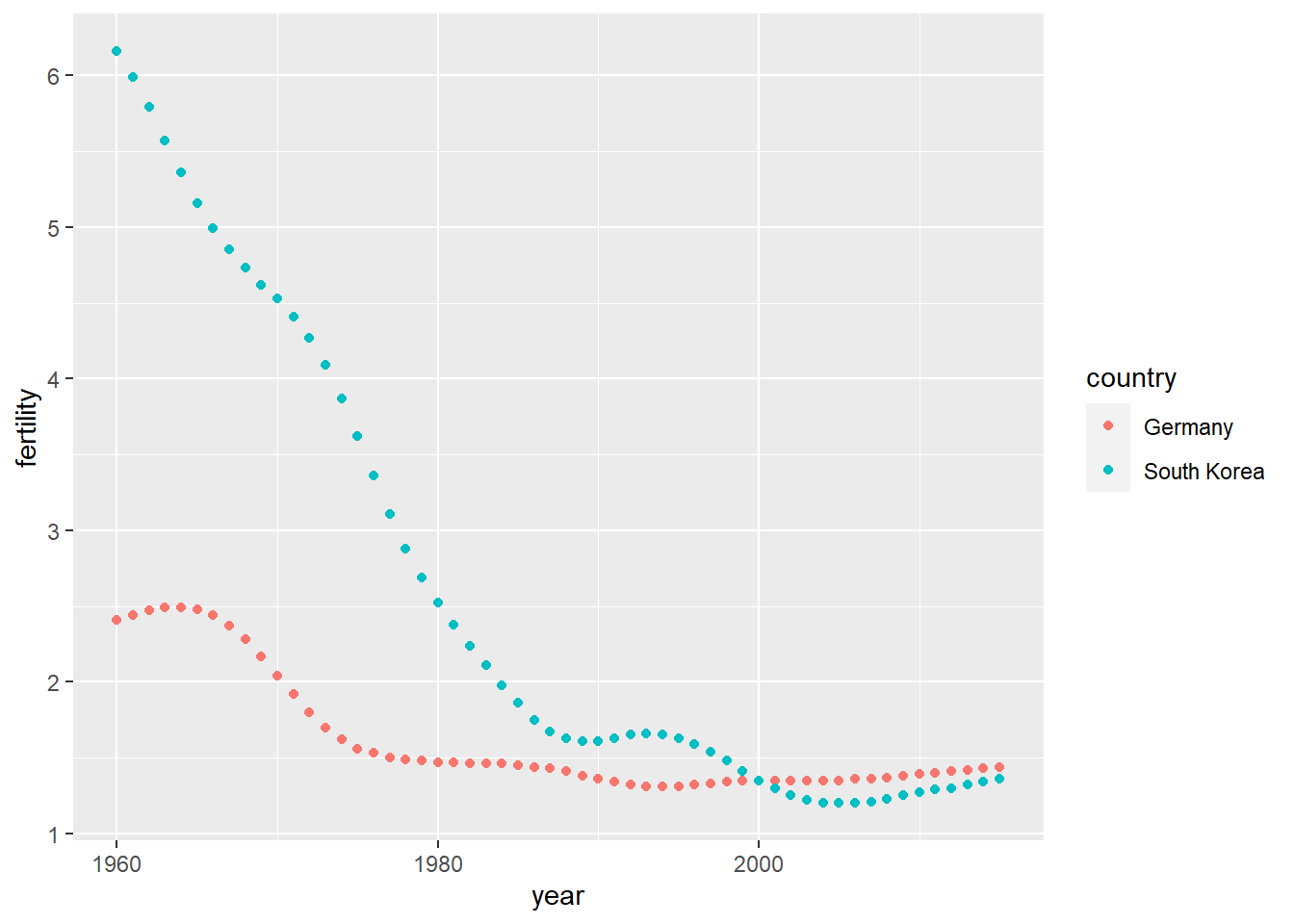

Plot showing South Korean fertility rate (green points) and German fertility rates (red points) from 1960 to approximately 2020. South Korean rates are much higher in 1960, while German rates are lower at around 2.5. Over time, German fertility rates decline to around 1.5, while South Korean drop from 6 to under 1.5 around 2000, remaining low through 2020.

`pivot_wider`

As we will see in later examples, it is sometimes useful for data wrangling purposes to convert tidy data into wide data. We often use this as an intermediate step in tidying up data. The pivot_wider function is basically the inverse of pivot_longer. The first argument is for the data, but since we are using the pipe, we don’t show it. The names_from = argument tells pivot_wider which variable will be used as the column names. The values_from = argument specifies which variable to use to fill out the cells:

new_wide_data <- new_tidy_data %>% pivot_wider(names_from = year, values_from = fertility)
dplyr::select(new_wide_data, country, `1960`:`1967`)

# A tibble: 2 × 9
  country     `1960` `1961` `1962` `1963` `1964` `1965` `1966` `1967`
  <chr>        <dbl>  <dbl>  <dbl>  <dbl>  <dbl>  <dbl>  <dbl>  <dbl>
1 Germany       2.41   2.44   2.47   2.49   2.49   2.48   2.44   2.37
2 South Korea   6.16   5.99   5.79   5.57   5.36   5.16   4.99   4.85

The following diagram can help remind you how these two functions work:

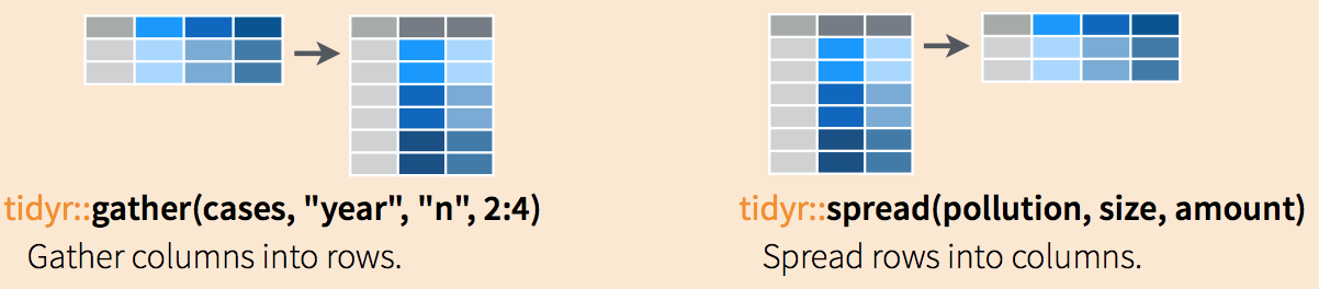
A plot showing a graphical depiction of pivoting wider and longer.

(Image courtesy of RStudio². CC-BY-4.0 license³. Cropped from original.)

`separate`

The data wrangling shown above was simple compared to what is usually required. In our example spreadsheet files, we include an illustration that is slightly more complicated. It contains two variables: life expectancy and fertility. However, the way it is stored is not tidy and, as we will explain, not optimal.

path <- system.file("extdata", package = "dslabs")

filename <- "life-expectancy-and-fertility-two-countries-example.csv"
filename <-  file.path(path, filename)

raw_dat <- read_csv(filename)
dplyr::select(raw_dat, 1:5)

# A tibble: 2 × 5
  country     `1960_fertility` `1960_life_expectancy` `1961_fertility`
  <chr>                  <dbl>                  <dbl>            <dbl>
1 Germany                 2.41                   69.3             2.44
2 South Korea             6.16                   53.0             5.99
# ℹ 1 more variable: `1961_life_expectancy` <dbl>

First, note that the data is in wide format. Second, notice that this table includes values for two variables, fertility and life expectancy, with the column name encoding which column represents which variable. Encoding information in the column names is not recommended but, unfortunately, it is quite common. We will put our wrangling skills to work to extract this information and store it in a tidy fashion.

We can start the data wrangling with the pivot_longer function, but we should no longer use the column name year for the new column since it also contains the variable type. We will call it key, the default, for now:

dat <- raw_dat %>% pivot_longer(-country, names_to = 'key', values_to = 'value')
head(dat)

# A tibble: 6 × 3
  country key                  value
  <chr>   <chr>                <dbl>
1 Germany 1960_fertility        2.41
2 Germany 1960_life_expectancy 69.3 
3 Germany 1961_fertility        2.44
4 Germany 1961_life_expectancy 69.8 
5 Germany 1962_fertility        2.47
6 Germany 1962_life_expectancy 70.0

The result is not exactly what we refer to as tidy since each observation (year-country combination) is associated with two, not one, rows. We want to have the values from the two variables, fertility and life expectancy, in two separate columns. The first challenge to achieve this is to separate the key column into the year and the variable type. Notice that the entries in this column separate the year from the variable name with an underscore:

dat$key[1:5]

[1] "1960_fertility"       "1960_life_expectancy" "1961_fertility"      
[4] "1961_life_expectancy" "1962_fertility"

Encoding multiple variables in a column name is such a common problem that the tidyverse package includes a function to separate these columns into two or more. Apart from the data, the separate function takes three arguments: the name of the column to be separated, the names to be used for the new columns, and the character that separates the variables. So, a first attempt at this is:

dat %>% separate(col = key, into = c("year", "variable_name"), sep = "_")

The function does separate the values, but we run into a new problem. We receive the warning Additional pieces discarded in 112 rows [3, 4, 7,...]. (Earlier versions may give the error Too many values at 112 locations:) and that the life_expectancy variable is truncated to life. This is because the _ is used to separate life and expectancy, not just year and variable name! We could add a third column to catch this and let the separate function know which column to fill in with missing values, NA, when there is no third value. Here we tell it to fill the column on the right:

dat %>% separate(key, into = c("year", "first_variable_name", "second_variable_name"), fill = "right")

# A tibble: 224 × 5
   country year  first_variable_name second_variable_name value
   <chr>   <chr> <chr>               <chr>                <dbl>
 1 Germany 1960  fertility           <NA>                  2.41
 2 Germany 1960  life                expectancy           69.3 
 3 Germany 1961  fertility           <NA>                  2.44
 4 Germany 1961  life                expectancy           69.8 
 5 Germany 1962  fertility           <NA>                  2.47
 6 Germany 1962  life                expectancy           70.0 
 7 Germany 1963  fertility           <NA>                  2.49
 8 Germany 1963  life                expectancy           70.1 
 9 Germany 1964  fertility           <NA>                  2.49
10 Germany 1964  life                expectancy           70.7 
# ℹ 214 more rows

However, if we read the separate help file, we find that a better approach is to merge the last two variables when there is an extra separation:

dat %>% separate(key, into = c("year", "variable_name"), extra = "merge")

# A tibble: 224 × 4
   country year  variable_name   value
   <chr>   <chr> <chr>           <dbl>
 1 Germany 1960  fertility        2.41
 2 Germany 1960  life_expectancy 69.3 
 3 Germany 1961  fertility        2.44
 4 Germany 1961  life_expectancy 69.8 
 5 Germany 1962  fertility        2.47
 6 Germany 1962  life_expectancy 70.0 
 7 Germany 1963  fertility        2.49
 8 Germany 1963  life_expectancy 70.1 
 9 Germany 1964  fertility        2.49
10 Germany 1964  life_expectancy 70.7 
# ℹ 214 more rows

This achieves the separation we wanted. However, we are not done yet. We need to create a column for each variable. As we learned, the pivot_wider function can do this:

dat %>%
  separate(key, c("year", "variable_name"), extra = "merge") %>%
  pivot_wider(names_from = variable_name, values_from = value)

# A tibble: 112 × 4
   country year  fertility life_expectancy
   <chr>   <chr>     <dbl>           <dbl>
 1 Germany 1960       2.41            69.3
 2 Germany 1961       2.44            69.8
 3 Germany 1962       2.47            70.0
 4 Germany 1963       2.49            70.1
 5 Germany 1964       2.49            70.7
 6 Germany 1965       2.48            70.6
 7 Germany 1966       2.44            70.8
 8 Germany 1967       2.37            71.0
 9 Germany 1968       2.28            70.6
10 Germany 1969       2.17            70.5
# ℹ 102 more rows

The data is now in tidy format with one row for each observation with three variables: year, fertility, and life expectancy.

`unite`

It is sometimes useful to do the inverse of separate, unite two columns into one. To demonstrate how to use unite, we show code that, although not the optimal approach, serves as an illustration. Suppose that we did not know about extra and used this command to separate:

dat %>%
  separate(key, c("year", "first_variable_name", "second_variable_name"), fill = "right")

# A tibble: 224 × 5
   country year  first_variable_name second_variable_name value
   <chr>   <chr> <chr>               <chr>                <dbl>
 1 Germany 1960  fertility           <NA>                  2.41
 2 Germany 1960  life                expectancy           69.3 
 3 Germany 1961  fertility           <NA>                  2.44
 4 Germany 1961  life                expectancy           69.8 
 5 Germany 1962  fertility           <NA>                  2.47
 6 Germany 1962  life                expectancy           70.0 
 7 Germany 1963  fertility           <NA>                  2.49
 8 Germany 1963  life                expectancy           70.1 
 9 Germany 1964  fertility           <NA>                  2.49
10 Germany 1964  life                expectancy           70.7 
# ℹ 214 more rows

We can achieve the same final result by uniting the second and third columns, then spreading the columns and renaming fertility_NA to fertility:

dat %>%
  separate(key, c("year", "first_variable_name", "second_variable_name"), fill = "right") %>%
  unite(variable_name, first_variable_name, second_variable_name) %>%
  pivot_wider(names_from = variable_name, values_from = value) %>%
  rename(fertility = fertility_NA)

# A tibble: 112 × 4
   country year  fertility life_expectancy
   <chr>   <chr>     <dbl>           <dbl>
 1 Germany 1960       2.41            69.3
 2 Germany 1961       2.44            69.8
 3 Germany 1962       2.47            70.0
 4 Germany 1963       2.49            70.1
 5 Germany 1964       2.49            70.7
 6 Germany 1965       2.48            70.6
 7 Germany 1966       2.44            70.8
 8 Germany 1967       2.37            71.0
 9 Germany 1968       2.28            70.6
10 Germany 1969       2.17            70.5
# ℹ 102 more rows

TRY IT

Run the following command to define the co2_wide object using the co2 data built in to R (see ?co2):

co2_wide <- data.frame(matrix(co2, ncol = 12, byrow = TRUE)) %>%
  setNames(1:12) %>%
  mutate(year = as.character(1959:1997))

Use the pivot_longer function to wrangle this into a tidy dataset. Call the column with the CO2 measurements co2 and call the month column month. Call the resulting object co2_tidy.

Plot CO2 versus month with a different curve for each year using this code:

co2_tidy %>% ggplot(aes(month, co2, color = year)) + geom_line()

If the expected plot is not made, it is probably because co2_tidy$month is not numeric:

class(co2_tidy$month)

Rewrite the call to pivot_longer using an argument that assures the month column will be numeric. Then make the plot.

What do we learn from this plot?

CO2 measures increase monotonically from 1959 to 1997.
CO2 measures are higher in the summer and the yearly average increased from 1959 to 1997.
CO2 measures appear constant and random variability explains the differences.
CO2 measures do not have a seasonal trend.

Now load the admissions data set, which contains admission information for men and women across six majors and keep only the admitted percentage column:

load(admissions)
dat <- admissions %>% dplyr::select(-applicants)

If we think of an observation as a major, and that each observation has two variables (men admitted percentage and women admitted percentage) then this is not tidy. Use the pivot_wider function to wrangle into tidy shape: one row for each major.

Now we will try a more advanced wrangling challenge. We want to wrangle the admissions data so that for each major we have 4 observations: admitted_men, admitted_women, applicants_men and applicants_women. The trick we perform here is actually quite common: first pivot_longer to generate an intermediate data frame and then pivot_wider to obtain the tidy data we want. We will go step by step in this and the next two exercises.

Use the pivot_longer function to create a tmp data.frame with a column containing the type of observation admitted or applicants. Call the new columns key and value.

Now you have an object tmp with columns major, gender, key and value. Note that if you combine the key and gender, we get the column names we want: admitted_men, admitted_women, applicants_men and applicants_women. Use the function unite to create a new column called column_name.
Now use the pivot_wider function to generate the tidy data with four variables for each major.
Now use the pipe to write a line of code that turns admissions to the table produced in the previous exercise.

Footnotes

If you have not installed this package already, you must use install.packages("tidyverse") prior to the library() call you see below.↩︎
https://github.com/rstudio/cheatsheets↩︎
https://github.com/rstudio/cheatsheets/blob/master/LICENSE↩︎

Readings

Your labs

Group project

Share your screen

Guiding Question

The tidyverse

Tidy data

Manipulating data frames

Adding a column with mutate

Subsetting with filter

Selecting columns with select

The pipe: %>%

Summarizing data

summarize

pull

Group then summarize with group_by

Sorting data frames

Nested sorting

Tibbles

Tibbles display better

Tibbles can be grouped

Create a tibble using tibble instead of data.frame

Applying more complex functions

The dot operator

The purrr package

Tidyverse conditionals

case_when

between

Reshaping data

pivot_longer

The pivot_longer arguments

pivot_wider

separate

unite

Footnotes

Adding a column with `mutate`

Subsetting with `filter`

Selecting columns with `select`

The pipe: `%>%`

`summarize`

`pull`

Group then summarize with `group_by`

Create a tibble using `tibble` instead of `data.frame`

`case_when`

`between`

`pivot_longer`

The `pivot_longer` arguments

`pivot_wider`

`separate`

`unite`